In reality nothing happens instantaneously, no matter how fast it appears to be.
When it comes to electronics, all signals are electromagnetic waves and they travel at the speed of light.
The wiring, circuit board material, or whatever the medium it is, affects the speed of light.
Wire or conductor structures that guide these waves are called transmission lines.
For non-magnetic media, this speed is:
$$v = \frac{c}{\sqrt{\epsilon_r}} = \frac{3×10^8}{\sqrt{\epsilon_r}}$$
This formula assumes a uniform (homogeneous) medium so it is not always simple to calculate the true propagation velocity.
For example, a track on the top surface of a circuit board has air above and fiberglass resin below. The effective permittivity will be somewhere between that of air (1) and fiberglass resin (4 to 5).
This post only discusses lossless transmission lines without any resistance.
Contents
When to Use Transmission Line Models?
Because the transmission line effects manifest themselves as delays they are only important for long lines.
Long in this case means electrically long, where the physical length depends on the signals of interest and the propagation medium.
Traditionally this means the line is at least 1/10 of a wavelength, which is equal to:
$$\lambda = \frac{v}{f} = \frac{3×10^8}{f\sqrt{\epsilon_r}}$$
In many cases it is more interesting to work with time-domain signals. In this case, an equivalent definition would be to state that an electrically long line has a propagation delay greater than 1/10 of the fastest signal transition time.
A line of length l has a propagation delay of:
$$t_d = \frac{l}{v} = \frac{l\sqrt{\epsilon_r}}{3×10^8}$$
Therefore, a signal with a 1 ns rise time would show transmission line effects for any line that has a delay of 0.1 ns or greater.
It needs to be said that the 1/10 rule is nothing special and sometimes 1/20 or even 1/2 is used.
Fundamentals
Characteristic Impedance
When analyzing transmission lines, the voltage and current are in general different at every point along each conductor due to propagation delay. In this case, the voltage and current are related by a constant ratio known as the characteristic impedance of the transmission line.
All conductors have both inductance and capacitance however characteristic impedance is slightly different, where it is actually defined by the per length inductance and capacitance. Remember, total line capacitance depends on length but because of the delay, the wave cannot actually “see” the entire line, so only the per length parameters matter.
For a lossless transmission line the characteristic impedance is:
$$Z_o = \sqrt{\frac{L}{C}}$$
This equation is inherently true of any conductor geometry. Therefore, lowering the capacitance necessarily increases the inductance and vice versa.
Per Length Parameters
The per length parameters that feed into the characteristic impedance equation can be calculated from electrostatic and magnetostatic equations for various geometries.
For instance, two parallel wires with radius r_w and separation s (with s >> r) are calculated as:
$$C = \frac{2\pi\epsilon}{\ln{\frac{s}{r_w}}} [F/m]$$
$$L = \frac{\mu}{\pi}\ln{\frac{s}{r_w}} [H/m]$$
Therefore, the characteristic impedance is:
$$Z_o = \frac{1}{\pi}\sqrt{\frac{\mu}{\epsilon}}\ln{\frac{s}{r_w}}$$
Parameters for Entire Length
For a line of length l, the total capacitance and inductance are:
$$C_t = Cl$$
$$L_t = Ll$$
This can be related to the propagation delay:
$$t_d = \sqrt{L_tC_t} = C_tZ_o = \frac{L_t}{Z_o}$$
Modeling Transmission Lines
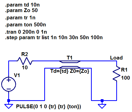
SPICE simulators, in this case LTSpice, typically provide a lossless transmission model. In LTSpice it’s called a “tline” where you define the time delay td and the characteristic impedance Zo. As we saw above, that uniquely defines the total inductance and capacitance. It is interesting to note that the actual length is unknown without knowing the propagation medium i.e. permittivity.
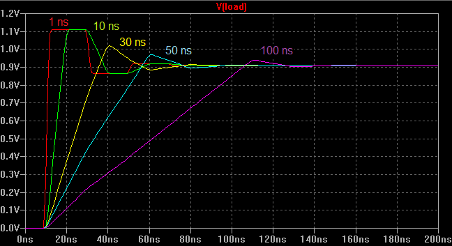
Below is an LTSpice schematic with a 10 ohm driver and a 100 ohm load, passing through a 50 ohm, 10 ns transmission line. As discussed earlier, transmission line models are necessary when the transition time of the signal is 1/10 the delay of the line or faster.
Below is the result for a 1 V pulse with different rise times; 1 ns, 10 ns, 30 ns, 50 ns and 100 ns. First of all, the pulse starts at 0 s but only appears at the load after 10 ns — this is the time delay of the transmission line.
For the fast signals there is noticeable ringing, but unlikely typical ringing it is completely square. This ringing is actually due to reflections moving back and forth through the line, taking 10 ns to travel there and back — this results in overshoot pulses lasting 20 ns. In the case of the slow signals, the reflections finish their trip before the source signal has finished settling. This results in the reflections having very little effect. In the case of the 100 ns rise time (delay of 1/10 of rise time) the overshoot is only 3%.